Hidden Markov Model ( HMM )

 Unraveling the Enigma: Exploring the Hidden  Markov Model

Introduction

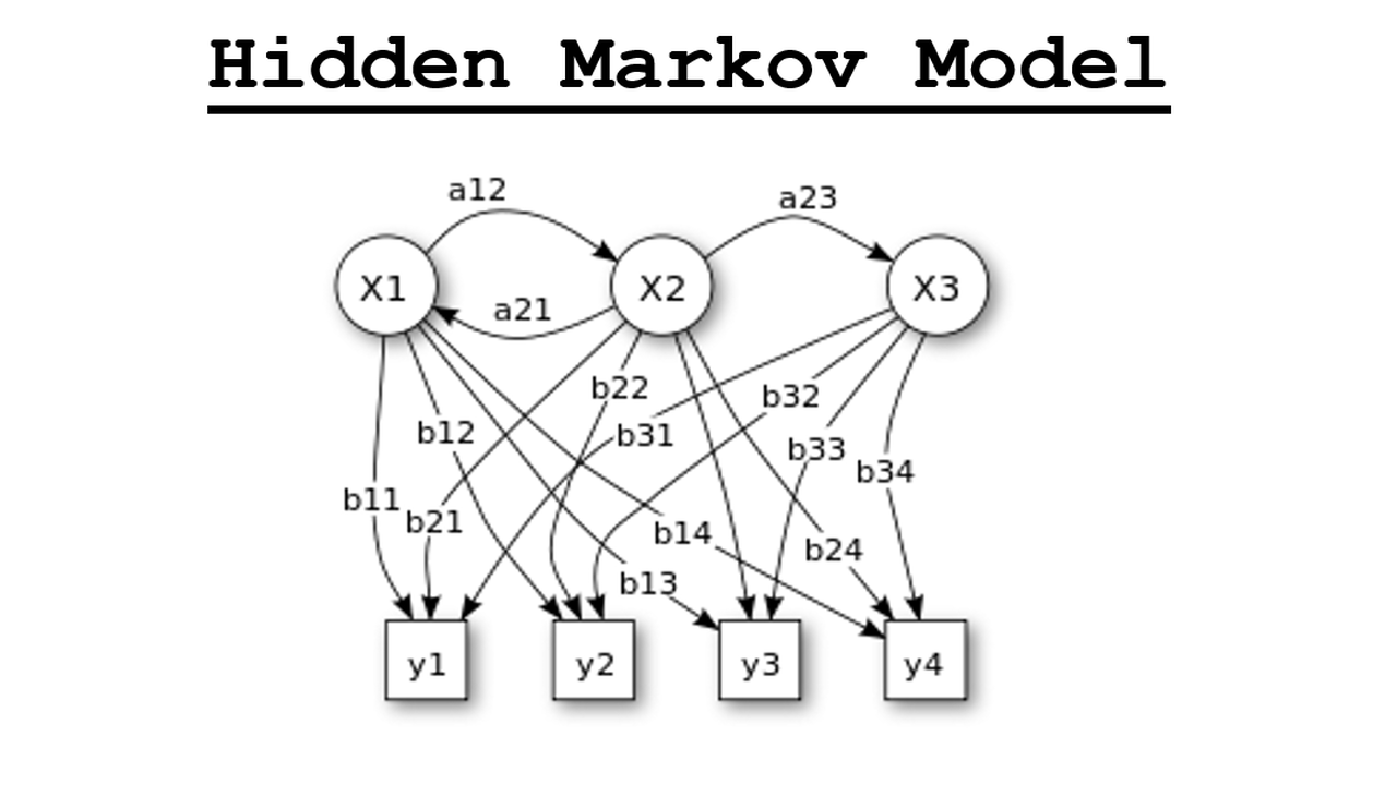
Hidden Markov Model is a probabilistic statistical model in machine learning which is used to describe the probability between a sequence of hidden and observed states. It is mainly used for prediction and classification.    

Fig 1: Hidden Markov Model

Terminology Decoded

Model:

It is a machine learning model that uses a dataset as its training dataset. A model's primary function in machine learning is to do a desired task by taking a dataset as a reference and preparing it as a ready-to-use algorithm so that when subsequent datasets are used, it will produce the proper output that it learned using the training dataset. A model might include several algorithms and employs the concept of learning. A model is employed for this purpose.

Hidden States:

Hidden states are variables that are unobservable( unmeasurable ) but are inferred or calculated based on observed data.

Observed States:

Observed states are variables that store the characteristics that are present in that dataset and may be directly measured. The observed states have an impact on the hidden states. 

Fig 2: Hidden States and Observation States

Transition Probability:

The probability that tracks the transfer of hidden states from one to another in a dataset is known as transition probability. The observed states determine the probability (value) of a label in a dataset changing its hidden state from one to another. 

Emission Probability:

Emission probability is a metric that tracks the possibility of each hidden state producing a certain combination of visible states. It measures the likelihood (value) of viewing specific states by analyzing and comprehending the links between concealed and visible states.

Fig 3: Transition and Emission Probabilities

Explanation

1. Labelled Dataset: First it begins with a labelled dataset in which each data point has an associated label. The HMM is trained using this dataset. This is also called as training data. The HMM examines the labelled dataset to determine the elements that impact or differentiate the labels. It seeks patterns and connections between the factors and the labels. 
2. Observed States: Factors that can be measured or observed directly are saved as observed states. Variables that capture the important measurements or attributes of the data points are often used to represent these observed states.
3. Hidden States: The observed states are utilized to figure out what the hidden states are. The underlying variables or phenomena that generate the seen data are represented by the hidden states. The labels or discrepancies between the labels in the dataset are caused by hidden states. They are not directly quantifiable and are saved using the label name or another representation.
4. Transition Probability: The transition probabilities explain the possibility of a concealed state shifting to another. These probabilities capture the dynamics or transitions between hidden states in an observation sequence. They are determined by analyzing the labelled dataset.
5. Emission Probability: Given a concealed state, the emission probabilities describe the likelihood of witnessing specific outputs or measurements. They represent the link between the concealed and observable states. These probabilities are also calculated using the labelled dataset analysis. Here measurements or observed data are outputs. 
6. Model Set-up: Once the transition and emission probabilities are calculated, a model is built around them. The training data is used by the HMM to learn the patterns and correlations between the hidden and seen states. This trained model can then be used to predict and classify new, previously unseen data.

  

Algorithm for Hidden Markov Model

1) Define the observation space and the state space 

• State Space: This is the set of all potential hidden states, which represent the system's underlying components or phenomena.
• Observation Space: This is the set of all conceivable observations that can be measured or witnessed directly.

2) Define the Initial State Distribution

The initial state distribution aids in determining the HMM's starting point. It gives the model a probability distribution over the possible hidden states, allowing it to start its analysis from a specific state depending on the probabilities.

3) Define the State Transition Probabilities  

These probabilities describe the chances of transitioning from one hidden state to another. It forms a transition matrix that captures the probability of moving between states.

4) Define the Observation Probabilities

These probabilities describe the possibility of each observation being generated from each concealed state. It generates an emission matrix that describes the likelihood of generating each observation from each state. 

5) Train the Model

Algorithms such as Baum-Welch and forward-backward are used to estimate the parameters of state transition probabilities and observation likelihoods. These algorithms alter the parameters iteratively based on the observed data until they converge.

6) Decode the Sequence of Hidden States

The Viterbi algorithm is used to compute the most likely sequence of hidden states based on the observable data. This sequence can be used to anticipate future observations, classify sequences, or find data patterns.

7) Evaluate the Model

The accuracy, precision, recall, and F1 score of the HMM can all be used to evaluate its performance. These metrics assess how successfully the model predicts or categorizes data.

Example of Hidden Markov Model

1) Establish the observation and state spaces

• State Space: Let's pretend we have three hidden states: "sunny," "cloudy," and "rainy." These are the many weather situations.
• Observation Space: In our case, the observations are "umbrella" and "sunglasses." These are the observable signs that can be used to forecast the weather.

2) Define the Initial State Distribution

We define the initial state distribution, which at the start assigns probability to each concealed state. For example, we may have a better chance of starting with a "sunny" day rather than "cloudy" or "rainy."

3) Determine the Probabilities of State Transition

We calculate the chances of switching between concealed states. For example, switching from "sunny" to "cloudy" may be more likely than transitioning from "sunny" to "rainy" or vice versa. A transition matrix captures these probability.

Step 4: Define the Probabilities of Observation

Given a specified hidden state, we assign probabilities to each observation. For example, if the weather is "sunny," the likelihood of needing sunglasses is high, whereas the likelihood of needing an umbrella is low. These probabilities are used to generate an emission matrix.

Step 5: Develop the Model

The model learns the parameters of the state transition probabilities and observation probabilities using a training dataset of labelled weather observations. It iteratively modifies these settings using techniques such as Baum-Welch until they converge.

Step 6: Decode the Hidden State Sequence

Given a set of observations, such as "umbrella" and "sunglasses," the Viterbi algorithm determines the most likely sequence of hidden states. Based on the observed data, this sequence depicts the projected weather conditions.

Step 7: Assess the Model

Metrics such as accuracy can be used to evaluate the performance of the weather prediction model. This entails comparing anticipated weather states to actual weather states to determine how well the model predicts.

Fig 4: Example of Hidden Markov Model

Real Time Applications of Hidden Markov Model

1. Music analysis
2. Gesture learning in human-robot interface
3. Speech recognition
4. Natural language processing( NLP )  

Investigating the Person Behind the Blog

If you want to discover more about me and my experience, please visit click on the below link to go to About Me section. More information about my history, interests, and the aim of my site may be found there.

I'm happy to share more useful stuff with you in the future, so stay tuned! Please do not hesitate to contact me if you have any queries or would like to connect.

Thank you for your continued support and for being a part of this incredible blogging community!"

Link to About Me